Historically, there are a lot of researches about data structure and algorithms. This is a core field of computer science from the past. I’m especially interested in hash table among them because it is simple data structure and widely used but there are a lot of inspiring ideas in hash table.
Today I found a good article about the speed and efficiency of hash table. And I heard that one of the probing algorithm called Robin Hood. It’s not new algorithm but I never heard of it. It’s simple but efficient comparing with linear open addressing algorithm. So I did a simple experiment for learning Robin Hood hashing.
Robin Hood hashing
First I need to describe about Robin Hood algorithm briefly. Both linear probing and Robin Hood can be used in open addressing algorithm. In open addressing, calculate the hash value the entry to be inserted and then search position from the index which is calculated by initial hash value. But if there are already a lot of entries in hash table, collision may be occurred and it causes further searching. It can deteriorate insertion performance.
According to this article, the key point of Robin Hood is the variance. It tries to make the distribution of insertion/delete time smaller. It means we can expect Robin Hood to probide roughly same performance every time I Put or Erase. How can it achieve?
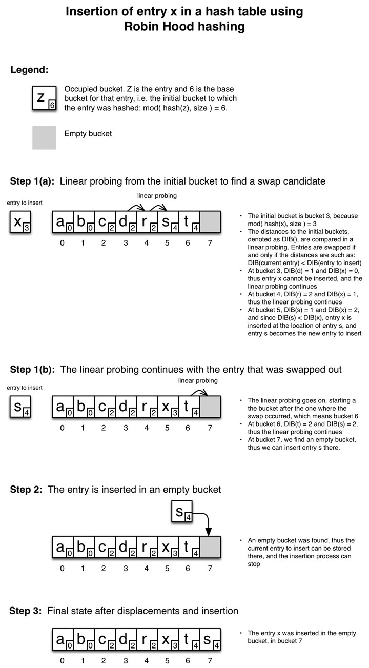
This is a great illustration of Robin Hood algorithm provided by Emmanuel Goossaert. According to this illustration, the algorithm is simple.
- Calculate the hash value and initial index of the entry to be inserted
- Search the position linearly
- While searching, the distance from initial index is kept which is called DIB(Distance from Initial Bucket)
- If we can find the empty bucket, we can insert the entry with DIB here
- If we encounter a entry which has less DIB than the one of the entry to be inserted, swap them.
In short, we can swap the entries if we find the entry which is stored nearer position from initial bucket than the entry to be inserted. We can regard the entry which has low DIB as rich, lucky one. So Robin Hood takes from who has and provide to who does not have. This is the derivation of Robin Hood algorithm.
Experiment
So I wrote a simple code to run experiment of Robin Hood.
The test case is
- Create 10000 fixed size hash table (for simplicity it cannot be resized)
- Running
PutandGetper each load factor target - Run above operation 20 times (epoch)
This is the distribution of elapsed time in each algorithm. Robin Hood aims to avoid high variance of lookup time. Surely Robin Hood time of insert and lookup is smaller than the one of linear probing.
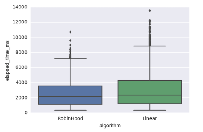
We can see low elapsed time even in high load factor case. The most efficient and stable case of
Robin Hood hashing looks around 0.5~0.6 load factor.

The experiment looks good but there is only one weird point. I also got the metrics of average DIB of every entries. But we cannot see any significant difference between linear and Robin Hood. So I’m not sure why the difference of the elapsed time variance is made for now. I’ll keep looking into the code and algorithm whether I might have made some mistake.