Bellman-Ford algorithm may be one of the most famous algorithms because every CS student should learn it in the university. Similarly to the previous post, I learned Bellman-Ford algorithm to find the shortest path to each router in the network in the course of OMSCS.
I want to try to make use of this chance to review my knowledge on the algorithm not to forget about it.
The normal version of Bellman-Ford algorithm is used to find the shortest path from a source node to every node in the target graph. A graph consists of multiple nodes and edges. For example, the following diagram shows the shortest path cost from the source node A.
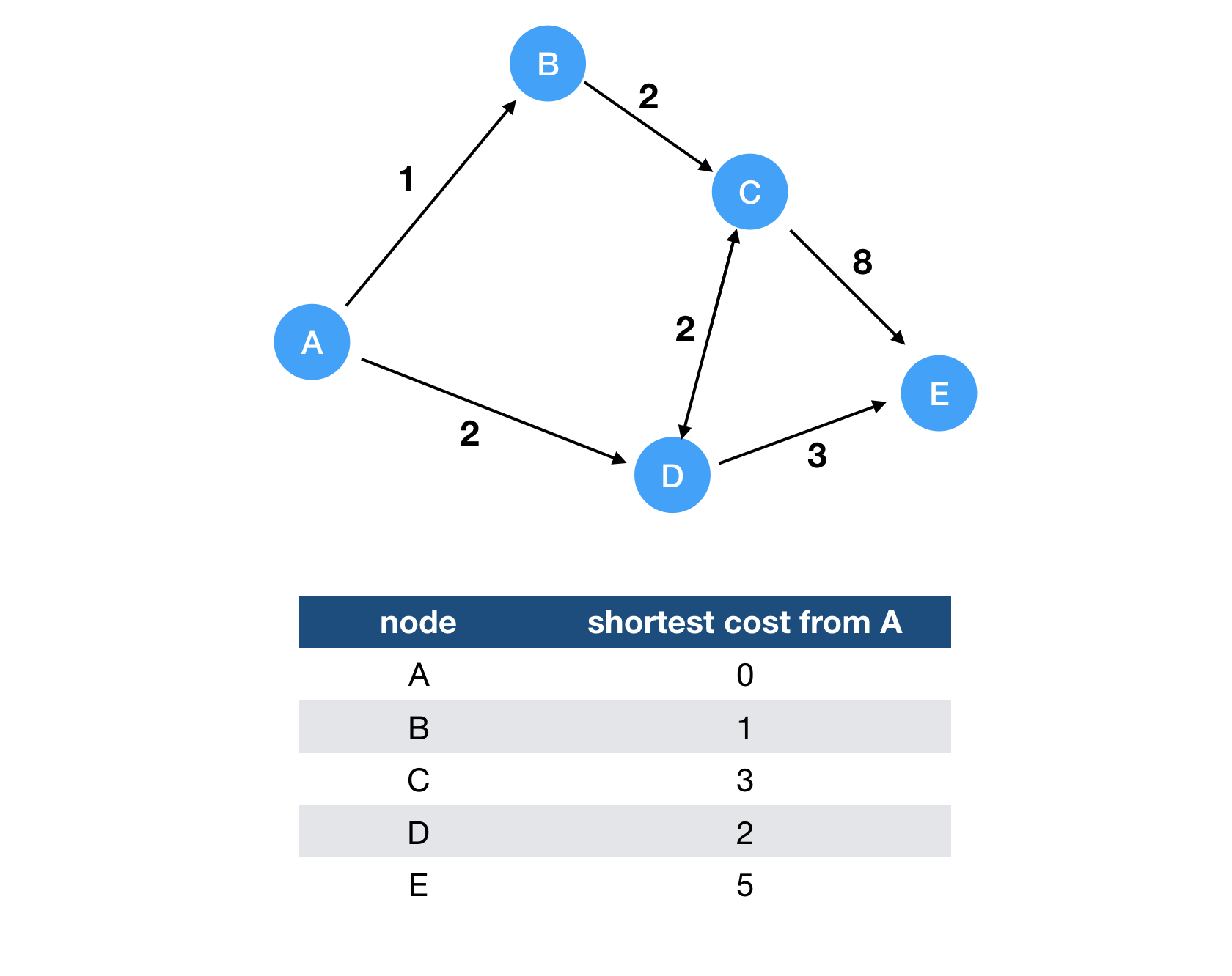
You can use the shortest path cost from the specified source node by using Bellman-Ford algorithm. Dijkstra’s algorithm is also a famous one to find the shortest path in the given graph. While Dijkstra’s algorithm is faster than Bellman-Ford algorithm, it’s versatile and can handle the case with some edges with negative costs. This is the simple code of Bellman-Ford algorithm.
Non Distributed Bellman-Ford Algorithm
# graph is defined as the dictionary from the source to target
# For example, the aforementioned graph is represented as
graph = {
  'A': {'B': 1, 'D': 2},
  'B': {'C': 2},
  'C': {'D': 2, 'E': 8},
  'D': {'E': 3},
  'E': {}
}

def bellman_ford(graph, source):
    # Initialize the distance vector from the source node.
    distances = {}
    for node in graph:
        distances[node] = float('inf')
    # Of course, we can reach the source node with zero cost.
    distances[source] = 0

    # Keep running the iteration until it converges at most the number of nodes.
    for i in range(len(graph)-1):
        for u in graph:
            for v in graph[u]: # For each neighbour of u
                if distances[u] + graph[u][v] < distances[v]:
                    distances[v] = distances[u] + graph[u][v]

    # Check for negative-weight cycles
    for u in graph:
        for v in graph[u]:
            assert distances[v] <= distances[u] + graph[u][v]

    return distances
Basically, it is necessary to visit all nodes and edges at most to converge. So the time complexity can be illustrated as follows. V is the number of nodes and E represents the total number of edges.
\[O(|V| \cdot |E|)\]Since we can make sure that the graph without any negative cycle converges, we can detect the negative cycle if it finds the shortest path furthermore. If a graph has a negative cycle, there is no shortest path because we can decrease the cost infinitely by visiting the negative cycle forever.
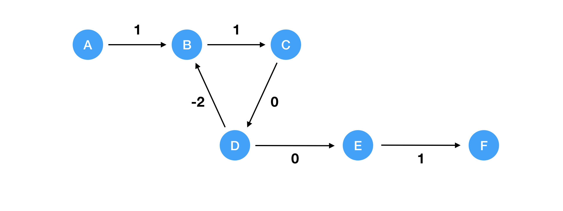
In this case, there is a negative cycle (B->C->D). Therefore, there is no shortest path from A->F because you can keep decreasing the cost by visiting B->C->D forever. So please keep in mind that Bellman-Ford algorithm cannot find the shortest path if the graph has a negative cycle.
Distributed Bellman-Ford Algorithm
A distributed version of Bellman-Ford algorithm is used to find the best routing path to send data packets between routers. Each router will get the routing table showing the shortest path to the destined router. But how? There is no central component to manage the routing table on the internet. That should be naturally treated in a distributed manner. This is the place where distributed Bellman-Ford algorithm comes up.
Distributed Bellman-Ford algorithm is also referred to as distance vector routing protocol. Each node gets the optimal routing table by exchanging routing table information each other. Since updating the routing table by applying the logic of Bellman-Ford algorithm, it’s also called Bellman-Fold algorithm. The message exchanged each other consists of the following information.
- Origin: The origin node the message is sent from.
- Routing Table: The routing table the origin node has at the time.
By exchanging this information, the optimal routing table will be obtained. Here is the pseudo like code to run the distributed Bellman-Ford algorithm.
class Node(object):
    def __init__(self, name):
        self.name = name
        self.routing_talbe = {}
        self.routing_table[self.name] = 0

    # message consists of
    # - origin
    # - routing_table
    def process_message(message):
        # Get the cost from this node to the origin node the message is sent from.
        cost = self.get_cost(self.name, message['origin'])
        # Traverse all nodes the origin node knows
        for u, c in message['origin'].routing_table.items():
            if u in self.routing_table:
                # Update this routing table according to the Bellman-Ford algorithm
                if cost + c < self.routing_table[u]:
                    self.routing_table[u] = cost + c
            else:
                # If this node does not know u, it should be included in the routing table.
                self.routing_table[u] = cost + c
The algorithm itself is simple. When a node receives a message, it traverses all nodes reachable from the origin node. If the current cost to the node is greater than the sum of cost to the origin and cost in the given routing table, it should be updated. Let’s take a look into how the algorithm progresses.
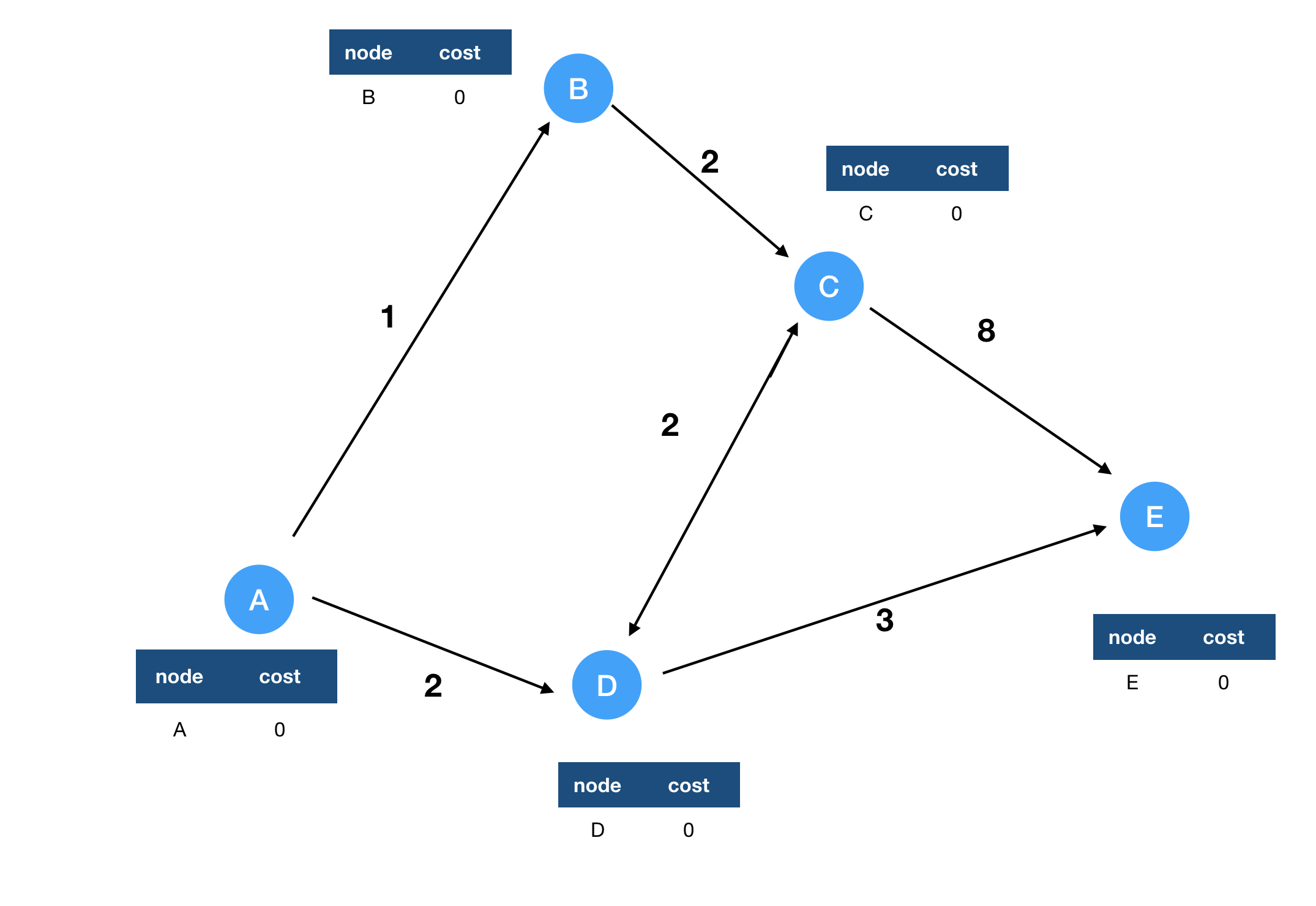
In the next step, node A receives a message from B and D including their routing tables. Then the routing table of A will look like this.
| node | cost |
|---|---|
| A | 0 |
| B | 1 |
| D | 2 |
Every other node processes the messages came from incoming neighbors similarly. Then the routing table will look like this overall.
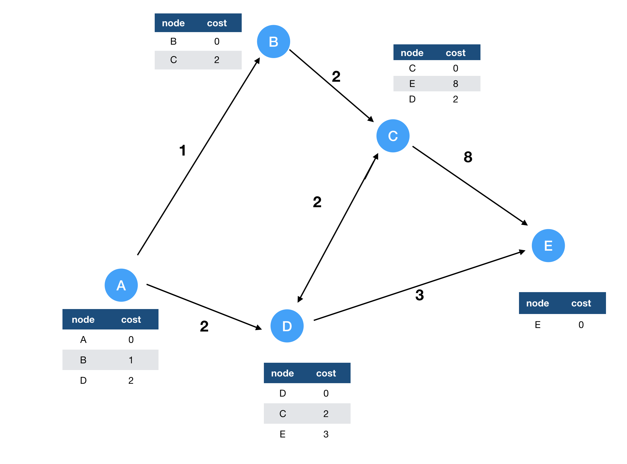
Since E does not have any outgoing links, its routing table is not updated. Other nodes which have outgoing links can receive the routing table information from its neighbors. Then the messages are sent to each other as long as its own routing table is updated. Here is the illustration after the next step.
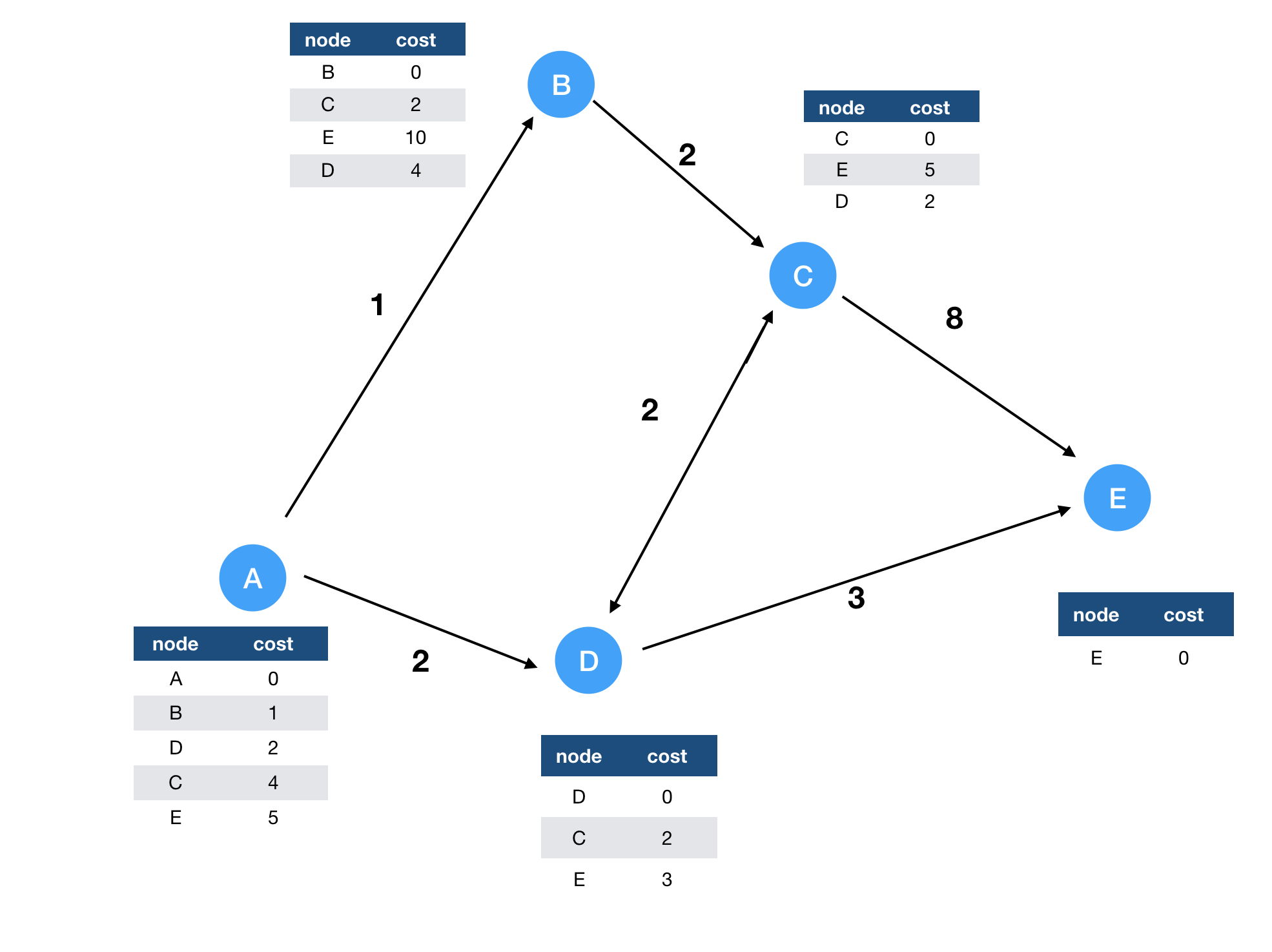
Since C gets a message from D routing to E, it knows it can reach to E via D with total cost 5. B also updates its routing table but it gets the non-optimal routing table from C. So it still does not know the optimal routing to E.
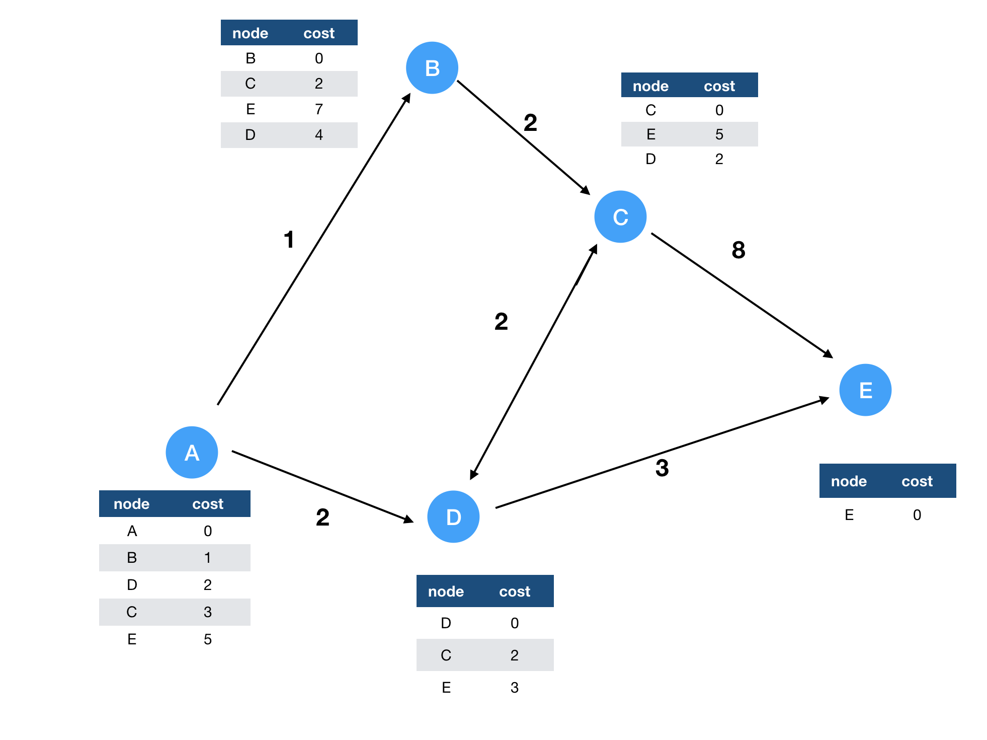
In this case, the routing table is converged as follows.
We need to take care of the case of the negative cycle. Unlikely with normal Bellman-Ford algorithm, distributed version cannot handle properly the negative cycle simply because it causes the infinite loop. Each node keeps sending the message each other as long as it sees the updates in its own routing table. If there is a negative cycle in the graph, the routing table is updated forever. In the normal case, there is an upper bound of the number of iterations. But the distributed algorithm does not have such limit so that a negative cycle in a graph can cause the infinite loop. We need to treat them carefully.
“Network Warrior”, Gary A. Donahue provides the concrete algorithm which is used in the real world. The book was helpful to refine my knowledge around the computer network.
Thanks!
Photo by Clint Adair on Unsplash