In general, visualization is an essential technique to understand what is happening. The software does not always provide informative metrics to us for debugging and inspection. We must get them visualized proactively. Notably, it is hard to investigate how a distributed program works without well-defined visualization tools due to the nature of its asynchronous and uncertainty. In this article, I’m going to demonstrate how to visualize the execution plan of Presto which is one of the most advanced distributed execution systems.
Environment
You can quickly try to run the following code by using docker-presto-cluster.
$ make run
The Presto cluster with version 318 is launched in your local machine. Please make sure to install the Presto CLI to run the query to the cluster. The instruction is here.
The following code connects to the local coordinator with specifying tpch catalog and tiny schema as default.
$ ./presto-cli-318-SNAPSHOT-executable.jar --server localhost:8080 --catalog tpch --schema tiny
First, let’s look at how to print the logical plan.
Logical Plan
EXPLAIN is a significant feature to print the logical plan used in various kind of implementations supporting SQL. Presto also shows the logical plan as default by using EXPLAIN. EXPLAIN (TYPE LOGICAL) does the same thing.
presto:tiny> explain select custkey, cnt from (select custkey, count(1) cnt from customer group by custkey) where cnt > 10;
                                                    Query Plan
------------------------------------------------------------------------------------------------------------------
 Output[custkey, cnt]
 │   Layout: [custkey:bigint, count:bigint]
 │   Estimates: {rows: ? (?), cpu: ?, memory: ?, network: ?}
 │   cnt := count
 └─ RemoteExchange[GATHER]
    │   Layout: [custkey:bigint, count:bigint]
    │   Estimates: {rows: ? (?), cpu: ?, memory: ?, network: ?}
    └─ Filter[filterPredicate = ("count" > BIGINT '10')]
       │   Layout: [custkey:bigint, count:bigint]
       │   Estimates: {rows: ? (?), cpu: ?, memory: ?, network: ?}
       └─ Aggregate(FINAL)[custkey]
          │   Layout: [custkey:bigint, count:bigint]
          │   Estimates: {rows: ? (?), cpu: ?, memory: ?, network: ?}
          │   count := count("count_16")
          └─ LocalExchange[HASH][$hashvalue] ("custkey")
             │   Layout: [custkey:bigint, count_16:bigint, $hashvalue:bigint]
             │   Estimates: {rows: ? (?), cpu: ?, memory: ?, network: ?}
             └─ RemoteExchange[REPARTITION][$hashvalue_17]
                │   Layout: [custkey:bigint, count_16:bigint, $hashvalue_17:bigint]
                │   Estimates: {rows: ? (?), cpu: ?, memory: ?, network: ?}
                └─ Project[]
                   │   Layout: [custkey:bigint, count_16:bigint, $hashvalue_18:bigint]
                   │   Estimates: {rows: ? (?), cpu: ?, memory: ?, network: ?}
                   │   $hashvalue_18 := "combine_hash"(bigint '0', COALESCE("$operator$hash_code"("custkey"), 0))
                   └─ Aggregate(PARTIAL)[custkey]
                      │   Layout: [custkey:bigint, count_16:bigint]
                      │   count_16 := count(*)
                      └─ TableScan[tpch:customer:sf0.01]
                             Layout: [custkey:bigint]
                             Estimates: {rows: 1500 (13.18kB), cpu: 13.18k, memory: 0B, network: 0B}
                             custkey := tpch:custkey
It prints the hierarchy of logical operations of the query.
Distributed Plan
To print the physical plan, which is a real execution plan of the distributed environment, you can specify the type DISTRIBUTED. A fragment represents a stage of the distributed plan. Presto scheduler schedules the execution by each stage, and stages can be run on separated instances.
presto:tiny> explain (type distributed) select custkey, cnt from (select custkey, count(1) cnt from customer group by custkey) where cnt > 10;
                                             Query Plan
----------------------------------------------------------------------------------------------------
 Fragment 0 [SINGLE]
     Output layout: [custkey, count]
     Output partitioning: SINGLE []
     Stage Execution Strategy: UNGROUPED_EXECUTION
     Output[custkey, cnt]
     │   Layout: [custkey:bigint, count:bigint]
     │   Estimates: {rows: ? (?), cpu: ?, memory: ?, network: ?}
     │   cnt := count
     └─ RemoteSource[1]
            Layout: [custkey:bigint, count:bigint]

 Fragment 1 [HASH]
     Output layout: [custkey, count]
     Output partitioning: SINGLE []
     Stage Execution Strategy: UNGROUPED_EXECUTION
     Filter[filterPredicate = ("count" > BIGINT '10')]
     │   Layout: [custkey:bigint, count:bigint]
     │   Estimates: {rows: ? (?), cpu: ?, memory: ?, network: ?}
     └─ Aggregate(FINAL)[custkey]
        │   Layout: [custkey:bigint, count:bigint]
        │   Estimates: {rows: ? (?), cpu: ?, memory: ?, network: ?}
        │   count := count("count_16")
        └─ LocalExchange[HASH][$hashvalue] ("custkey")
           │   Layout: [custkey:bigint, count_16:bigint, $hashvalue:bigint]
           │   Estimates: {rows: ? (?), cpu: ?, memory: ?, network: ?}
           └─ RemoteSource[2]
                  Layout: [custkey:bigint, count_16:bigint, $hashvalue_17:bigint]

 Fragment 2 [SOURCE]
     Output layout: [custkey, count_16, $hashvalue_18]
     Output partitioning: HASH [custkey][$hashvalue_18]
     Stage Execution Strategy: UNGROUPED_EXECUTION
     Project[]
     │   Layout: [custkey:bigint, count_16:bigint, $hashvalue_18:bigint]
     │   Estimates: {rows: ? (?), cpu: ?, memory: ?, network: ?}
     │   $hashvalue_18 := "combine_hash"(bigint '0', COALESCE("$operator$hash_code"("custkey"), 0))
     └─ Aggregate(PARTIAL)[custkey]
        │   Layout: [custkey:bigint, count_16:bigint]
        │   count_16 := count(*)
        └─ TableScan[tpch:customer:sf0.01, grouped = false]
               Layout: [custkey:bigint]
               Estimates: {rows: 1500 (13.18kB), cpu: 13.18k, memory: 0B, network: 0B}
               custkey := tpch:custkey
IO
We may sometimes want to focus on the IO of the query. Like which table is the query reading? TYPE IO brings us the information around the table and schemas the query reads in JSON format.
presto:tiny> explain (type io) select custkey, cnt from (select custkey, count(1) cnt from customer group by custkey) where cnt > 10;
           Query Plan
---------------------------------
 {
   "inputTableColumnInfos" : [ {
     "table" : {
       "catalog" : "tpch",
       "schemaTable" : {
         "schema" : "sf0.01",
         "table" : "customer"
       }
     },
     "columnConstraints" : [ ]
   } ]
 }
(1 row)
Graphviz
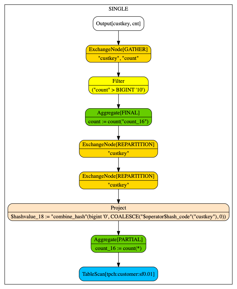
The printed information in the console is basically sufficiently useful, but we want to make it better in terms of the visibility. You can use the format option to print in the format compatible with Graphviz.
presto:tiny> explain (format graphviz) select custkey, cnt from (select custkey, count(1) cnt from customer group by custkey) where cnt > 10;
                                                                                         Query Plan
--------------------------------------------------------------------------------------------------------------------------------------------------------------------------------------------
 digraph logical_plan {
 subgraph cluster_graphviz_plan {
 label = "SINGLE"
 plannode_1[label="{Output[custkey, cnt]}", style="rounded, filled", shape=record, fillcolor=white];
 plannode_2[label="{ExchangeNode[GATHER]|\"custkey\", \"count\"}", style="rounded, filled", shape=record, fillcolor=gold];
 plannode_3[label="{Filter|(\"count\" \> BIGINT '10')}", style="rounded, filled", shape=record, fillcolor=yellow];
 plannode_4[label="{Aggregate[FINAL]|count := count(\"count_16\")\n}", style="rounded, filled", shape=record, fillcolor=chartreuse3];
 plannode_5[label="{ExchangeNode[REPARTITION]|\"custkey\"}", style="rounded, filled", shape=record, fillcolor=gold];
 plannode_6[label="{ExchangeNode[REPARTITION]|\"custkey\"}", style="rounded, filled", shape=record, fillcolor=gold];
 plannode_7[label="{Project|$hashvalue_18 := \"combine_hash\"(bigint '0', COALESCE(\"$operator$hash_code\"(\"custkey\"), 0))\n}", style="rounded, filled", shape=record, fillcolor=bisque];
 plannode_8[label="{Aggregate[PARTIAL]|count_16 := count(*)\n}", style="rounded, filled", shape=record, fillcolor=chartreuse3];
 plannode_9[label="{TableScan[tpch:customer:sf0.01]}", style="rounded, filled", shape=record, fillcolor=deepskyblue];
 }
 plannode_1 -> plannode_2;
 plannode_2 -> plannode_3;
 plannode_3 -> plannode_4;
 plannode_4 -> plannode_5;
 plannode_5 -> plannode_6;
 plannode_6 -> plannode_7;
 plannode_7 -> plannode_8;
 plannode_8 -> plannode_9;
 }

(1 row)
Of course, it is not so useful as it is. Copy and paste it in the file (plan.dot). You can use the dot tool to convert the text format in the image. Please see here about the installation.
$ dot -Tpng plan.dot > plan.png
This is the graph generated by dot. Although it is a little cumbersome to create the image file like this, it is more informative and intuitive to grasp the overview of the dependencies between each operator.
You can use Graphviz format for distributed plan too. It’s fun to see how these two plans can be different from each other. Let’s try to make use of the tool to pursue more performant distributed queries.
Thanks!
Image by Andrew Martin from Pixabay