The outbreak of the novel coronavirus disease (Covid-19) brought considerable turmoil all around the world. Although the number of new patients in the mainland Child is restrained, the other countries are still struggling with the increasing number of new cases. I sincerely hope the situation will get better soon. At the same time, I am interested in how the spread of infectious diseases such as Covid-19 can happen. Is there anything we know about the mechanism of the spread disease?
I have found there is a simple mathematical model named SIR model describing the structure of how the infectious disease. The assertion by the model is so interesting to me even it is simple to explain. This post aims to deliver an overview of the SIR model and the outcome of my simulation by using the dataset of Covid-19.
Please refer to the repository used in this simulation for more detail.
- What is SIR model
- Simulation with COVID-19 data
- SIR Illustration
- Wrap Up
What is SIR model
SIR model is a kind of compartmental model describing the dynamics of infectious disease. You may wonder why it is called the “compartmental model.” The model divides the population into compartments. Each compartment is expected to have the same characteristics. SIR represents the three compartments segmented by the model.
- Susceptible
- Infectious
- Recovered
Susceptible is a group of people who are vulnerable to exposure with infectious people. They can be patient when the infection happens. The group of infectious represents the infected people. They can pass the disease to susceptible people and can be recovered in a specific period. Recovered people get immunity so that they are not susceptible to the same illness anymore. SIR model is a framework describing how the number of people in each group can change over time.
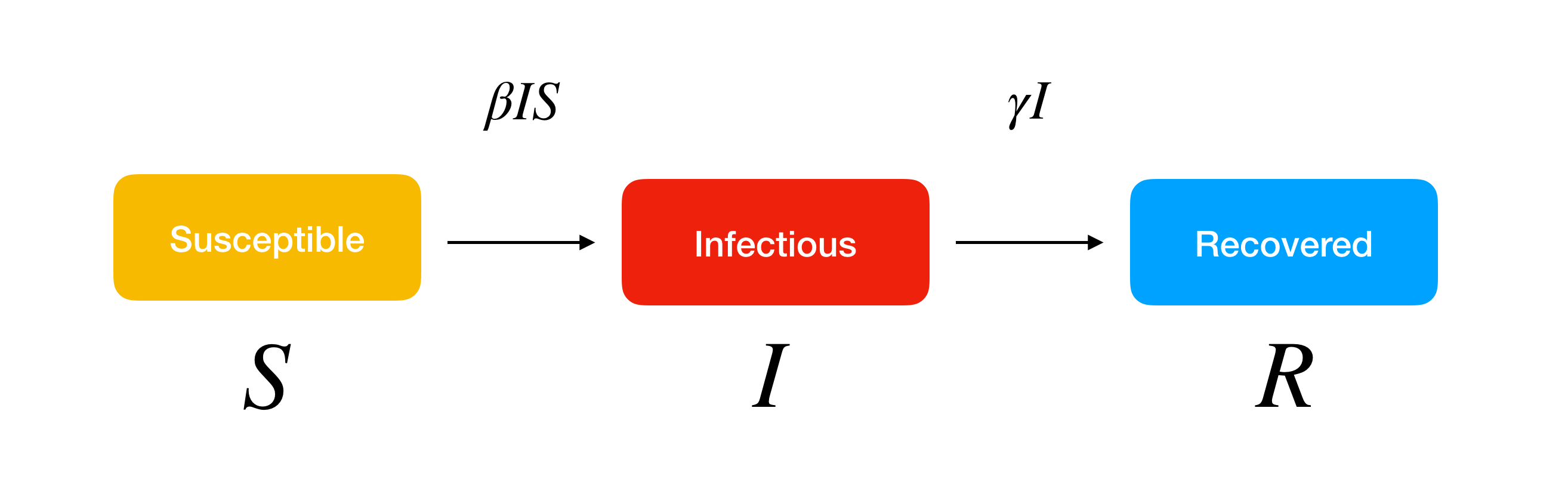
SIR model allows us to describe the number of people in each compartment with the ordinary differential equation. \(\beta\) is a parameter controlling how much the disease can be transmitted through exposure. It is determined by the chance of contact and the probability of disease transmission. \(\gamma\) is a parameter expressing how much the disease can be recovered in a specific period. Once the people are healed, they get immunity. There is no chance for them to go back susceptible again.
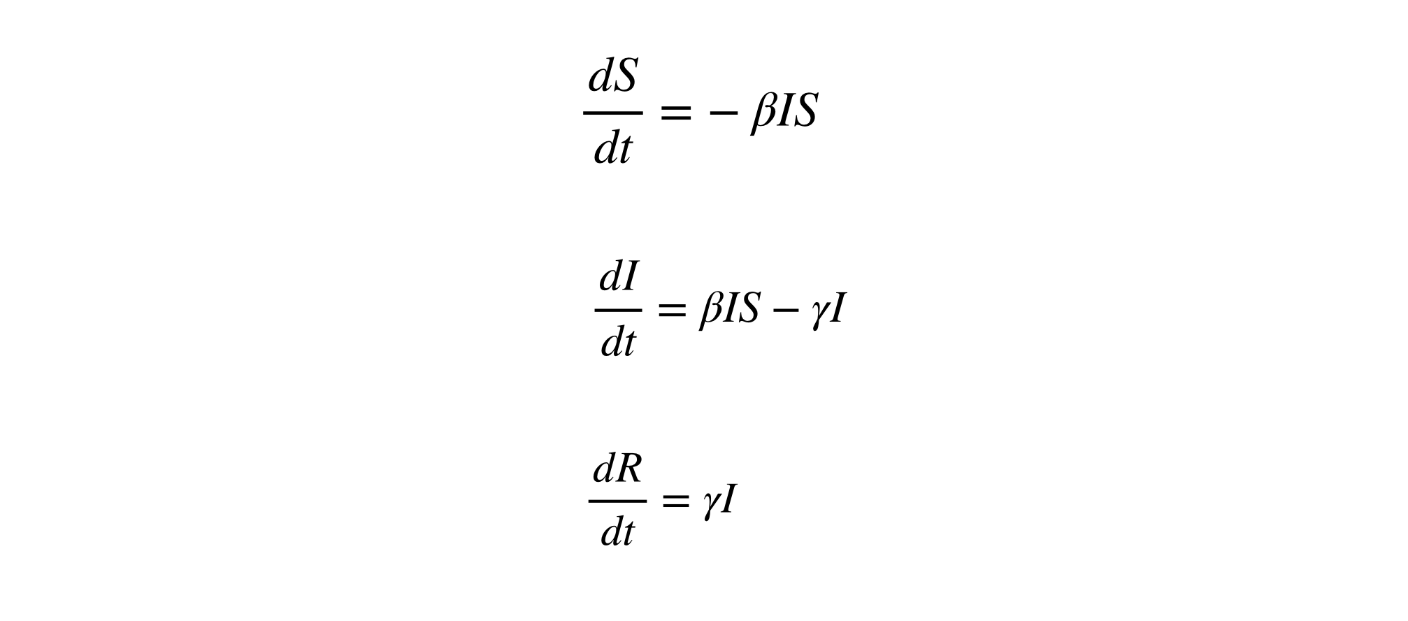
We do not consider the effect of the natural death or birth rate because the model assumes the outstanding period of the disease is much shorter than the lifetime of the human. It lets us know the importance of knowing two parameters, \(\beta\) and \(\gamma\). When we can estimate the two values, there are several insights derived from it. If the \(D\) is the average days to recover from infectious, it is derived from \(\gamma\).
\begin{equation} D = \frac{1}{\gamma} \end{equation}
Also, we can estimate the nature of the disease in terms of the power of infection.
\begin{equation} R_0 = \frac{\beta}{\gamma} \end{equation}
It is called a basic reproduction number. \(R_0\) is the average number of people infected from one other person. If it is high, the probability of pandemic is also higher. The number is also used to estimate the herd immune threshold (HIT). If the basic reproduction number multiplied by the percentage of non-immune people (susceptible) is equal to 1, it indicates the balanced state. The number of infectious people is constant. Assume the proportion of immune people is \(p\), the stable state can be formulated as follows.
\begin{equation}
R_0 (1 - p) = 1 \rightarrow
1 - p = \frac{1}{R_0} \rightarrow
p_c = 1 - \frac{1}{R_0}
\end{equation}
Therefore, \(p_c\) is the HIT to stop the spread of the infectious disease. We can stop the outbreak by vaccinating the population to increase herd immunity.
The video provided by 3Blue1Brown is also a great resource to learn the SIR model visually.
We have got the basics of the SIR model and what each metric means in terms of the dynamics of the spread of the infectious disease. Now it’s time to apply the model to COVID-19 case.
Simulation with COVID-19 data
The data source I have used in this experiment is available in HDX. We can download the number of cases which is:
What we are going to do is estimate the \(\beta\) and \(\gamma\) to fit the SIR model with the actual confirmed cases (the number of infectious people). To solve the ordinary differential equation like the SIR model, we can use solve_ivp function in scipy module.
import numpy as np
import pandas as pd
from scipy.integrate import solve_ivp
from scipy.optimize import minimize
import matplotlib.pyplot as plt
from datetime import timedelta, datetime

START_DATE = {
  'Japan': '1/22/20',
  'Italy': '1/31/20',
  'Republic of Korea': '1/22/20',
  'Iran (Islamic Republic of)': '2/19/20'
}

class Learner(object):
    def __init__(self, country, loss):
        self.country = country
        self.loss = loss

    def load_confirmed(self, country):
      """
      Load confirmed cases downloaded from HDX
      """
      df = pd.read_csv('data/time_series_19-covid-Confirmed.csv')
      country_df = df[df['Country/Region'] == country]
      return country_df.iloc[0].loc[START_DATE[country]:]

    def extend_index(self, index, new_size):
        values = index.values
        current = datetime.strptime(index[-1], '%m/%d/%y')
        while len(values) < new_size:
            current = current + timedelta(days=1)
            values = np.append(values, datetime.strftime(current, '%m/%d/%y'))
        return values

    def predict(self, beta, gamma, data):
        """
        Predict how the number of people in each compartment can be changed through time toward the future.
        The model is formulated with the given beta and gamma.
        """
        predict_range = 150
        new_index = self.extend_index(data.index, predict_range)
        size = len(new_index)
        def SIR(t, y):
            S = y[0]
            I = y[1]
            R = y[2]
            return [-beta*S*I, beta*S*I-gamma*I, gamma*I]
        extended_actual = np.concatenate((data.values, [None] * (size - len(data.values))))
        return new_index, extended_actual, solve_ivp(SIR, [0, size], [S_0,I_0,R_0], t_eval=np.arange(0, size, 1))

    def train(self):
        """
        Run the optimization to estimate the beta and gamma fitting the given confirmed cases.
        """
        data = self.load_confirmed(self.country)
        optimal = minimize(
            loss,
            [0.001, 0.001],
            args=(data),
            method='L-BFGS-B',
            bounds=[(0.00000001, 0.4), (0.00000001, 0.4)]
        )
        beta, gamma = optimal.x
        new_index, extended_actual, prediction = self.predict(beta, gamma, data)
        df = pd.DataFrame({
            'Actual': extended_actual,
            'S': prediction.y[0],
            'I': prediction.y[1],
            'R': prediction.y[2]
        }, index=new_index)
        fig, ax = plt.subplots(figsize=(15, 10))
        ax.set_title(self.country)
        df.plot(ax=ax)
        fig.savefig(f"{self.country}.png")
The loss function used in the optimization process was the root mean squared error (RMSE).
def loss(point, data):
    """
    RMSE between actual confirmed cases and the estimated infectious people with given beta and gamma.
    """
    size = len(data)
    beta, gamma = point
    def SIR(t, y):
        S = y[0]
        I = y[1]
        R = y[2]
        return [-beta*S*I, beta*S*I-gamma*I, gamma*I]
    solution = solve_ivp(SIR, [0, size], [S_0,I_0,R_0], t_eval=np.arange(0, size, 1), vectorized=True)
    return np.sqrt(np.mean((solution.y[1] - data)**2))
How can we decide the initial values of compartments? SIR model expects the susceptible to be homogenous, well-mixed, and accessible to each other. Setting the whole population in the country is not realistic for sure. I roughly infer the number of susceptible people in the compartment 15000. The number was determined by the rough inference of the max quantity of susceptible people except for mainland China. And also, it’s determined by the computational capacity. (Over 1 million susceptible people did not allow me to complete the calculation in a short time). The initial infectious people were 2 for every country, although the start of the outbreak is different.
SIR Simulation
I have run the estimation process for four countries.
- Japan
- South Korea
- Italy
- Iran
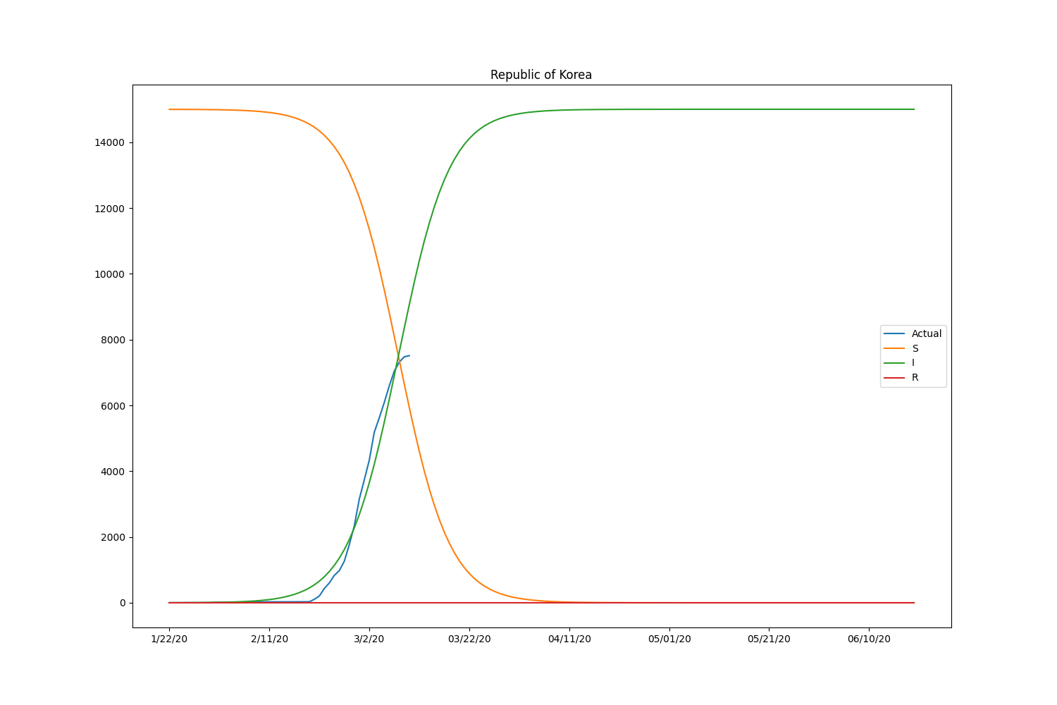
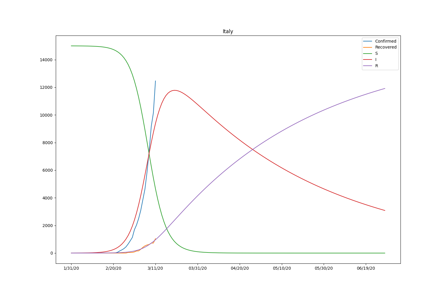
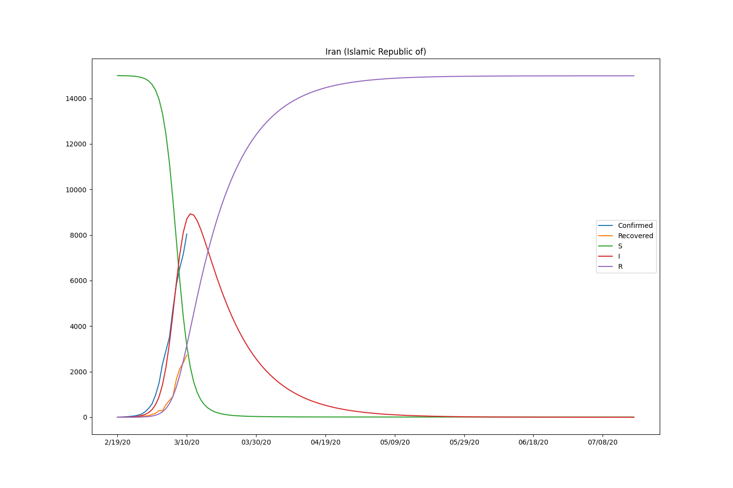
They are the major countries suffering from the CODIV-19 outbreak. The following images illustrate how the number of the compartment can be changed over time, according to the SIR model.
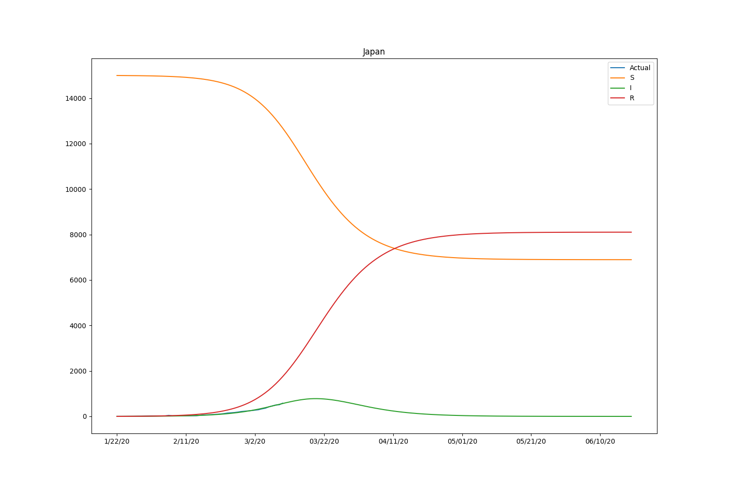
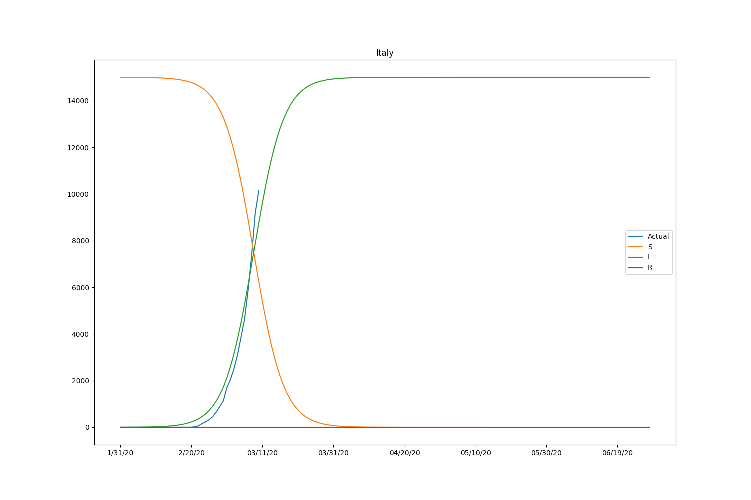
| Country | \(\beta\) | \(\gamma\) | \(R_0\) |
|---|---|---|---|
| Japan | 0.00002856 | 0.29819303 | 0.00009578 |
| South Korea | 0.00001297 | 0.00000001 | 1297.49430758 |
| Italy | 0.00001582 | 0.00000001 | 1581.92377423 |
| Iran | 0.00006294 | 0.39999237 | 0.00015735 |
Hmm, with this parameter, the model is well-fitting to Japanese case but not suitable for other countries. We may need to adjust the initial setting by countries or take into account the number of recovered people. Let’s modify the loss function to consider the recovered people too. The data is also available in HDX.
def loss(point, data, recovered):
    size = len(data)
    beta, gamma = point
    def SIR(t, y):
        S = y[0]
        I = y[1]
        R = y[2]
        return [-beta*S*I, beta*S*I-gamma*I, gamma*I]
    solution = solve_ivp(SIR, [0, size], [S_0,I_0,R_0], t_eval=np.arange(0, size, 1), vectorized=True)
    l1 = np.sqrt(np.mean((solution.y[1] - data)**2))
    l2 = np.sqrt(np.mean((solution.y[2] - recovered)**2))
    # Put more emphasis on recovered people
    alpha = 0.1
    return alpha * l1 + (1 - alpha) * l2
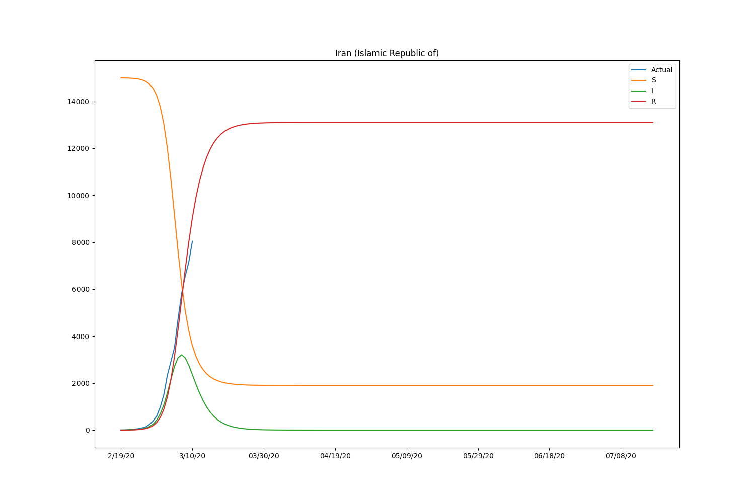
Here is the result, including the recovered people.
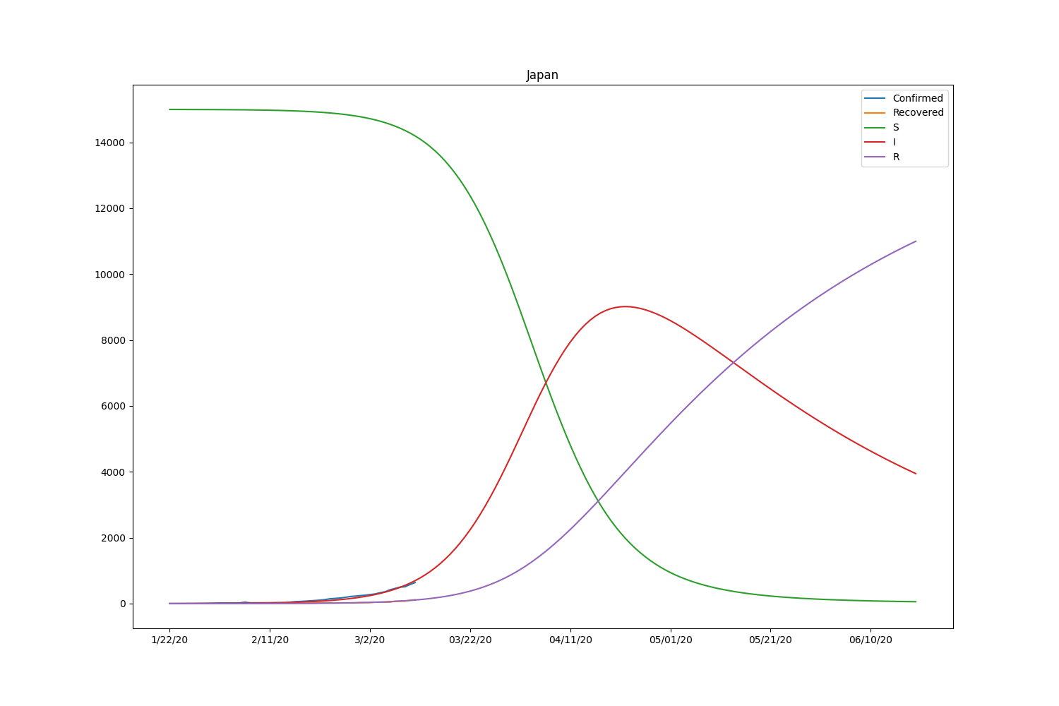
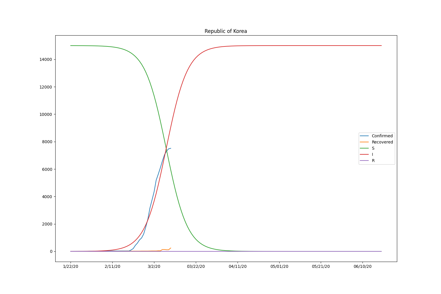
| Country | \(\beta\) | \(\gamma\) | \(R_0\) |
|---|---|---|---|
| Japan | 0.00000927 | 0.01837935 | 0.00050458 |
| South Korea | 0.00001298 | 0.00000001 | 1297.76738269 |
| Italy | 0.00001713 | 0.01414756 | 0.00121065 |
| Iran | 0.00003974 | 0.08023309 | 0.00049526 |
Now the SIR model is well-fitting the actual data for both confirmed and recovered cases. The \(R_0\) of South Korea is significantly higher than in other countries. That might be caused by the relatively lower rate of recovery of the country. Based on the result, the \(R_0\) is pretty lower than it should be. It will be roughly 2-5 (SARS) according to the statistics of the past infectious diseases if the calculation is correct. Probably, the assumption of the initial values can be wrong or fail to find the global minimum in the optimization process.
Wrap Up
Anyway, one important thing here is that it’s not the official one. Not surprisingly, it can be wrong. This experiment is done for satisfying my interest in the SIR model fitting to the COVID-19 dataset to see the dynamics of the spread of new disease-causing the widespread pandemic. I would be glad if this article is helpful for those who are also interested in the mechanism of the spread of infectious disease in general.
To learn more about SIR model and mechanism of the spread of infectious disease, please take a look at the “Stochastic Epidemic Models With Inference (Lecture Notes in Mathematics). Although the book is heavy to read through, there is no better book to learn the basic of the mechanism from my point of view.

Last but not least, please be sure to wash your hand regularly and keep away from the crowded area as general guidance says. I hope the outbreak will be over soon.
The full code used in this simulation is available in GitHub.
References
- Compartmental models in epidemiology
- Novel Coronavirus (COVID-19) Cases
- COVID-19 from WHO
- Lewuathe/COVID19-SIR
- Stochastic Epidemic Models With Inferenc (Lecture Notes in Mathematics)
Image by Gerd Altmann from Pixabay