Dataflow analysis is a technique to collect information about the possible state that the program can take at each point of the flow of the program. This analysis lets us know, for instance, which variables are alive at the specific point of the program or how many times a variable is used in the program.
Many compilers use this technique for fundamental transformation, such as register allocation and optimization of the program. However, to this day, I have thought data flow analysis is complicated and messy to learn. There are many types of analysis, and each one has a specific algorithm to complete the analysis.
But this time, I have acquired the categorization of four major types of data flow analysis. We can write down the code for dataflow analysis mechanically by using this categorization. It is always fun to understand things that look tough at first. If you are interested in how the significant dataflow analysis works and eager to write the code for that, this article is for you.
Control Flow Graph
A control flow graph (CFG) provides us the basis for this type of analysis. We can do the majority type of data flow analysis on this data structure by iteratively walking through the basic blocks in the graph. For example, we have the following C/C++ program.
int x = 5;
int y = 1;
while (x != 1) {
  y = x * y;
  x -= 1;
}
We can abstractly represent this program by using the CFG as follows.
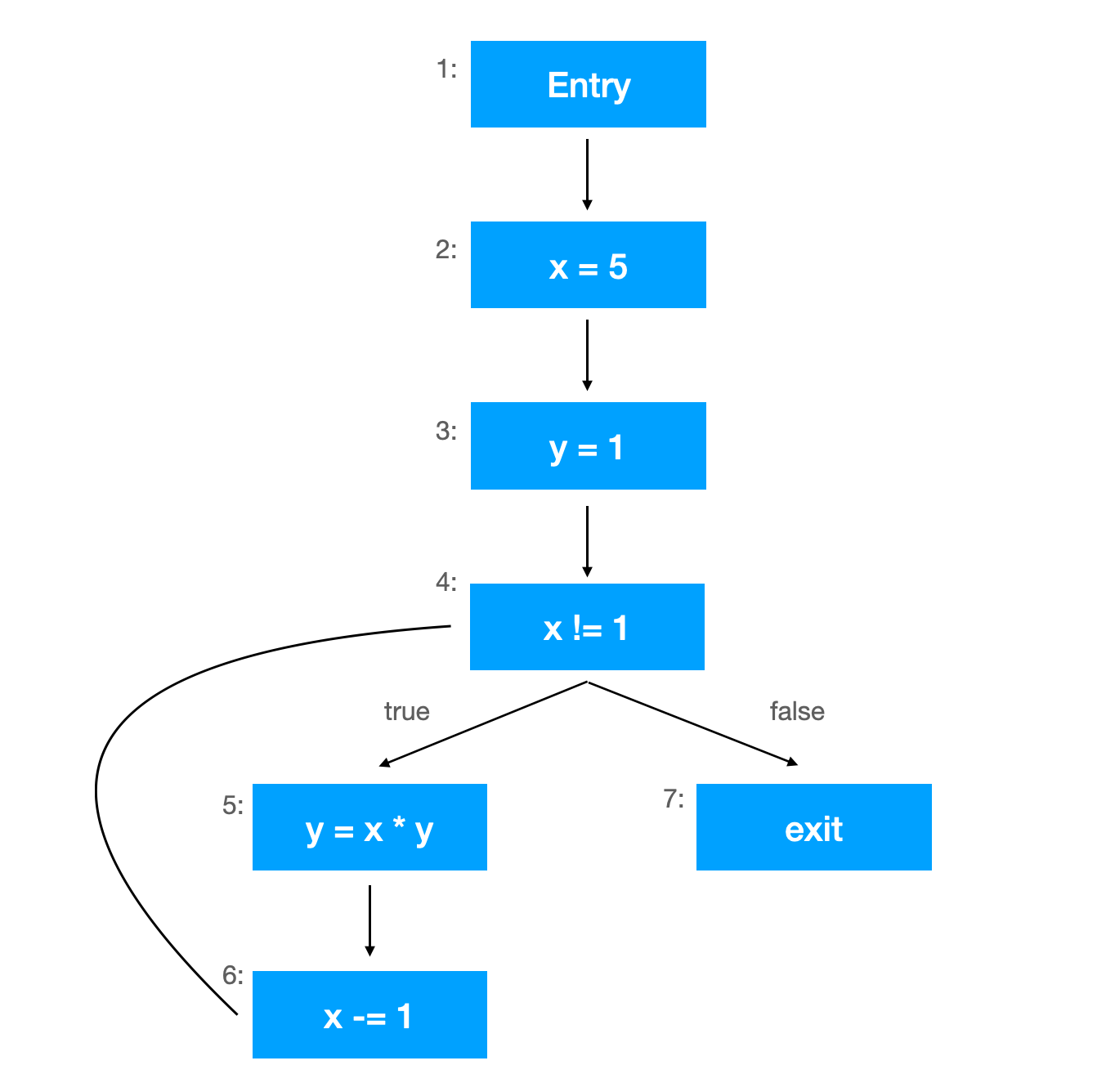
Each blue block represents a code line, and basic blocks are the blue blocks until it reaches the end of the program or branch condition.
We can accomplish the following four types of data flow analysis by using this CFG.
Let’s take a look at how the reaching definition goes as an example.
Reaching Definitions
Reaching definition analysis clarifies which assignments (definition) have been made and not overwritten for each program point.
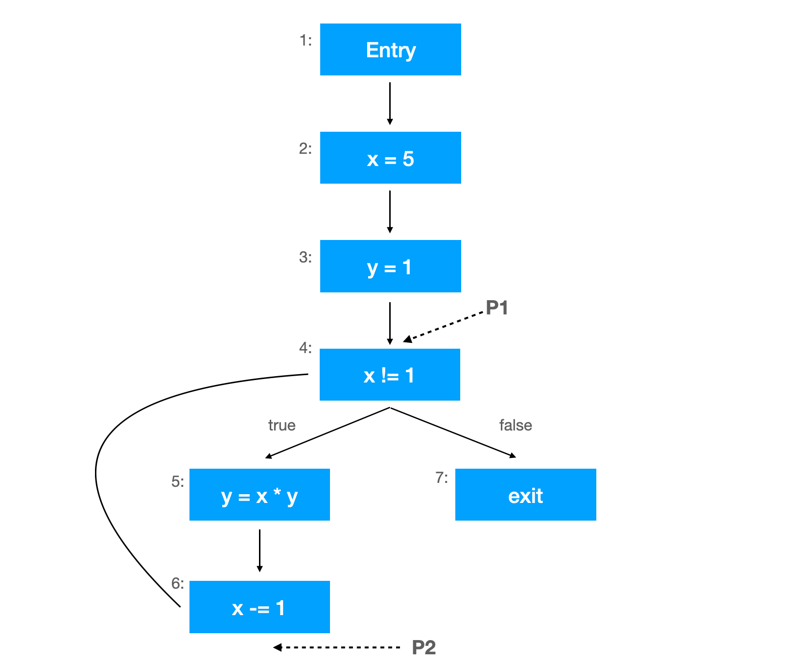
At the program point P1, for example, the assignment x = 5 reaches. It means the value assigned by x = 5 is alive at that point. On the other hand, the value is not active anymore at the point of P2 because x -= 1 overwrites the value for x. This analysis helps us find the usage of uninitialized variables in the program.
We can easily see which variable definition reaches that point at a glance. But how can we accomplish the same thing programmatically? Here comes the iterative algorithm.
Iterative Algorithm
We can describe the pseudo-code for the algorithm to complete this type of analysis as follows.
for n in nodes:
  IN[n] = N/A
  OUT[n] = N/A

while IN[] and OUT[] has been changed:
  for n in nodes:
    IN[n]= union of OUT[n'] for all predecessors of n
    OUT[n] = (IN[n] - KILL[n]) + GEN[n]
IN[] and OUT[] are the set collecting the fact at the program point. IN[] is for the fact at the entry of the control graph node, OUT[] is for the exit side. For example, if a definition x = 5 is reaching at the entry of node 4, IN[4] should contain x = 5.
KILL[] is a set of definitions overwritten by the node. GEN[] contains definitions assigned by that node. We should be able to get the collection of reaching definitions for each node in the graph if we run the program it converges.
Formal Operation
You may notice that the algorithm’s core consists of only two lines, collecting the union of OUT of predecessors and calculating the OUT set for each node. This operation can be mathematically described.
$ \text{IN[n]} = \bigcup_{n’ \in \text{pred(n)}} \text{OUT[n’]} $
$ \text{OUT[n]} = (\text{IN[n]} - \text{KILL[n]}) \cup \text{GEN[n]} $
These formulas remind us that the iteration goes forward from the predecessor to the node. We can calculate the input of the node from the output set of predecessors, and the node’s output is based on the input and what type of assignment the node does. This type of algorithm is categorized as a type of FORWARD analysis algorithm.
You can also see that the node’s input is collected from the union of the output of predecessors. It indicates that the fact satisfied in one of the predecessors can also be satisfied in the node. This type of analysis is called the MAY type of analysis because it does not require all the predecessors’ satisfaction.
As you may already notice, it looks like we can have other types of dataflow analysis. Can we construct the BACKWARD and MUST type of analysis in this manner?
Yes, we can.
Four Patterns of Major Dataflow Analysis
The following table lists the patterns we categorize the four dataflow analysis introduced at the beginning of the post.
| MAY | MUST | |
|---|---|---|
| FORWARD | Reaching Definition | Available Expressions |
| BACKWARD | Live Variables | Very Busy Expressions |
Although we omit the detail and meaning of each dataflow analysis here, you can get how the algorithm for them looks like. For instance, We can write the formula of available expression systematically:
$ \text{IN[n]} = \bigcap_{n’ \in \text{pred(n)}} \text{OUT[n’]} $
$ \text{OUT[n]} = (\text{IN[n]} - \text{KILL[n]}) \cup \text{GEN[n]} $
In short, we can replace the part of the formula according to the category the analysis falls into. MAY uses union operator (\(\bigcup\)), MUST uses intersection operator (\(\bigcap\)). For the forward analysis, the input is computed from the output of predecessors while the backward analysis gets the output from the input of successors. That’s it. These four algorithms should not show much difference.
Dataflow analysis seems complicated at a glance. But if you install this table in your brain, you can quickly write down the algorithm mechanically.