Previously I described how to implement custom WebGL operation in TensorFlow.js. In the post, you would learn how to write a fragment shader program to execute your own tensor manipulation in parallel.
According to the guide, once I implemented a fast fourier transform ops in TensorFlow.js that is now merged into master. FFT is a good example to show how parallelism of WebGL accelerates the execution of tensor computation simply. In this article, I’m going to show you the concrete example of WebGL implementation that computes FFT.
What is the Fast Fourier Transform?
Fast fourier transform is an algorithm to execute the fourier transform efficiently. Fourier transform is a computation that decomposes a function in time-series into frequencies. Actually, a video provided by 3 Blue 1 Brown was the best video to understand what fourier transform does quickly.
Mathematically, fourier transform can treat the continuous value but computers do not. Hence, the algorithm used by computers to calculate fourier transform is called discrete fourier transform (DFT). DFT converts finite samples of time-series data into the finite collection of frequencies. The input and output should have the same length and they both can be complex numbers in general.
Let’s suppose we have an input with complex numbers, \(\{x_n\} = x_0, x_1, \dots , x_{N-1}\) and the output of DFT would be \(\{X_k\} = X_0, X_1, \dots , X_{N-1}\). The output is considered as the frequencies which make of the original input. DFT is defined as follows.
\begin{equation} X_k = \sum_{n=0}^{N-1} x_n e^{-\frac{2\pi i}{N}kn} \end{equation}
\(e\) is the base of natural logarithm. \(i\) is an imaginary number so the result will be the complex number. For example, let’s say we have a time series data with 4 elements.
\begin{equation} x = \begin{pmatrix} x_0 \\ x_1 \\ x_2 \\ x_3 \end{pmatrix} = \begin{pmatrix} 1 \\ 2-i \\ -i \\ -1+2i \end{pmatrix} \end{equation}
Then we can calculate the frequencies as follows.
\begin{equation}
X =
\begin{pmatrix}
X_0 \\ X_1 \\ X_2 \\ X_3
\end{pmatrix}
=
\begin{pmatrix}
e^{-2\pi i \cdot 0 \cdot 0/ 4} + e^{-2\pi i \cdot 0 \cdot 1 / 4} (2-i) + e^{-2\pi i \cdot 0 \cdot 2 / 4} (-i) + e^{-2\pi i \cdot 0 \cdot 3 / 4}(-1+2i) \\
e^{-2\pi i \cdot 1 \cdot 0/ 4} + e^{-2\pi i \cdot 1 \cdot 1 / 4} (2-i) + e^{-2\pi i \cdot 1 \cdot 2 / 4} (-i) + e^{-2\pi i \cdot 1 \cdot 3 / 4}(-1+2i) \\
e^{-2\pi i \cdot 2 \cdot 0/ 4} + e^{-2\pi i \cdot 2 \cdot 1 / 4} (2-i) + e^{-2\pi i \cdot 2 \cdot 2 / 4} (-i) + e^{-2\pi i \cdot 2 \cdot 3 / 4}(-1+2i) \
e^{-2\pi i \cdot 3 \cdot 0/ 4} + e^{-2\pi i \cdot 3 \cdot 1 / 4} (2-i) + e^{-2\pi i \cdot 3 \cdot 2 / 4} (-i) + e^{-2\pi i \cdot 3 \cdot 3 / 4}(-1+2i)
\end{pmatrix}
=
\begin{pmatrix}
2 \\ -2-2i \\ -2i \\ 4+4i
\end{pmatrix}
\end{equation}
There must be no difficulty to understand the calculation itself. Besides, as you may already notice, the DFT algorithm is simply expressed as the matrix multiplication. Please take a look into the following equation.
\begin{equation}
X =
\begin{pmatrix}
X_0 \\ X_1 \\ X_2 \\ X_3
\end{pmatrix}
=
\begin{pmatrix}
\omega^{0 \cdot 0} && \omega^{0 \cdot 1} && \omega^{0 \cdot 2} && \omega^{0 \cdot 3} \
\omega^{1 \cdot 0} && \omega^{1 \cdot 1} && \omega^{1 \cdot 2} && \omega^{1 \cdot 3} \
\omega^{2 \cdot 0} && \omega^{2 \cdot 1} && \omega^{2 \cdot 2} && \omega^{2 \cdot 3} \
\omega^{3 \cdot 0} && \omega^{3 \cdot 1} && \omega^{3 \cdot 2} && \omega^{3 \cdot 3} \
\end{pmatrix}
\begin{pmatrix}
x_0 \\ x_1 \\ x_2 \\ x_3
\end{pmatrix}
\end{equation}
FFT in WebGL Platform
Let’s assume \(\omega = e^{-2\pi i/ N}\). An input data with N elements can be converted by NxN complex matrix. Here comes the tensor calculation. Matrix multiplication is one of the most frequently used operations in TensorFlow so that it can be done pretty efficiently thanks to the sophisticated implementations. One pitfall we need to pay attention to is that we need to support multiplication for complex values. Current matrix multiplication operator in TensorFlow.js does not support complex value. That’s why I created another kernel implementation just for fourier transform in TensorFlow.js.
Here is the WebGL kernel to compute fourier transform. TensorFlow.js calculate the fourier transform for real number and imaginary number separately. Due to the difference between the multiplication for real number and an imaginary number, unaryOpComplex function can have two type of implementation.
export const COMPLEX_FFT = {
  REAL: 'return real * expR - imag * expI;',
  IMAG: 'return real * expI + imag * expR;'
};

export class FFTProgram implements GPGPUProgram {
  variableNames = ['real', 'imag'];
  outputShape: number[];
  userCode: string;

  constructor(op: string, inputShape: [number, number], inverse: boolean) {
    const innerDim = inputShape[1];
    this.outputShape = inputShape;

    const exponentMultiplierSnippet =
        inverse ? `2.0 * ${Math.PI}` : `-2.0 * ${Math.PI}`;
    const resultDenominator = inverse ? `${innerDim}.0` : '1.0';

    this.userCode = `
      const float exponentMultiplier = ${exponentMultiplierSnippet};

      float unaryOpComplex(float real, float expR, float imag, float expI) {
        ${op}
      }

      float mulMatDFT(int batch, int index) {
        float indexRatio = float(index) / float(${innerDim});
        float exponentMultiplierTimesIndexRatio =
            exponentMultiplier * indexRatio;

        float result = 0.0;

        for (int i = 0; i < ${innerDim}; i++) {
          // x = (-2|2 * PI / N) * index * i;
          // This is corresponding to omega explained previously.
          float x = exponentMultiplierTimesIndexRatio * float(i);
          float expR = cos(x);
          float expI = sin(x);
          float real = getReal(batch, i);
          float imag = getImag(batch, i);

          result +=
              unaryOpComplex(real, expR, imag, expI) / ${resultDenominator};
        }

        return result;
      }

      void main() {
        ivec2 coords = getOutputCoords();
        // The input tensor is always reshaped into two dimentional tensor.
        setOutput(mulMatDFT(coords[0], coords[1]));
      }
    `;
  }
}
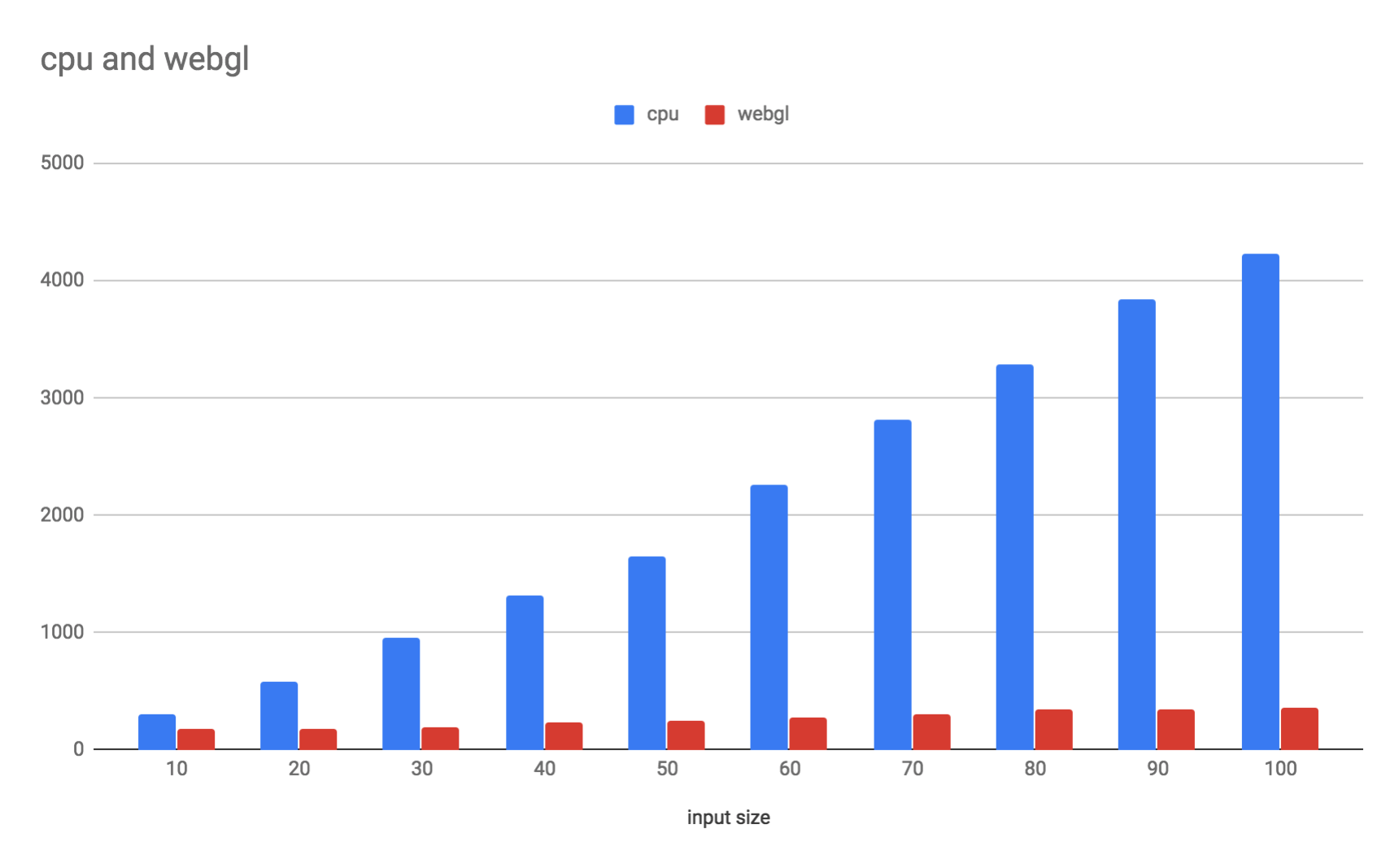
Honestly, there is no special thing in this implementation. It’s just a matrix multiplication supporting complex value. The algorithm is not even fast fourier transform such as Cooley–Tukey algorithm but it’s much faster because it’s accelerated by the high parallelism of GPU. Here is the result of micro-benchmark in my environment, Chrome: 71.0.3578.98 and macOS 10.13.6.
<html>
<head>
  <script src="https://cdn.jsdelivr.net/npm/@tensorflow/[email protected]/dist/tf.min.js"></script>
  <script type='text/javascript'>
    tf.setBackend('webgl');

    const nums = [1, 2, 3, 4, 5, 6, 7, 8, 9, 10];
    const results = nums.map(n => {
      const tensors = [];
      const start = performance.now();
      for (let i = 0; i < 100; i++) {
        const real = tf.ones([10, n * 10]);
        const imag = tf.ones([10, n * 10]);
        const input = tf.complex(real, imag);
        const res = tf.spectral.fft(input);
        res.dataSync();
      }
      return performance.now() - start;
    });
    console.log(results);
  </script>
</head>
</html>
You can see the WebGL implementation achieves a much better result than CPU implementation in terms of the speed and stability eve we increased the size of the input. If you want to learn more about TensorFlow.js and underlying technologies, “Deep Learning in the Browser” is a good resource to learn that kind of thing. That covers the latest technologies to run a deep learning algorithm in modern web browsers.

And of course, let’s try to implement your own kernel implementation for WebGL.
Thanks!